Article Text

Statistics from Altmetric.com
Introduction
Imagine you are assessing a patient with visual difficulties or optic disc swelling. After a bedside visual field examination with waggling fingers and even a red hatpin, you decide that there is an abnormality. After requesting quantified visual field tests, the patient returns with a black and white printout with numbers (eg, Humphrey fields) or coloured lines on a sheet (eg, Goldmann fields). Where is the report you ask? There is none!
Static perimetry uses flashing stationary lights. This can be automated (eg, evenly spaced points on a grid) or manual (eg, as a small part of Goldmann test: detailed later). The Humphrey field analyser is by far the most commonly used for automated static perimetry, although there are also other machines such as Octopus and Henson. Later, we describe in detail the interpretation of Humphrey perimetry.
Kinetic perimetry uses a moving illuminated target and is done either manually (eg, Goldmann) or on an automated machine (eg, Octopus). Goldmann machines are no longer manufactured, being slowly replaced by Octopus machines. Nevertheless, Goldmann remains the most commonly used kinetic perimetry, and so we use this here to illustrate interpretation of kinetic fields. The principles for interpreting Goldmann also apply to results from Octopus machines.
It is beyond the scope of this paper to cover the neuroanatomical localisation of visual field defects. Instead we recommend two excellent recent reviews.1 ,2 Skilled interpretation of visual field tests requires a good grasp and application of this prior knowledge.
Useful aspects of eye anatomy
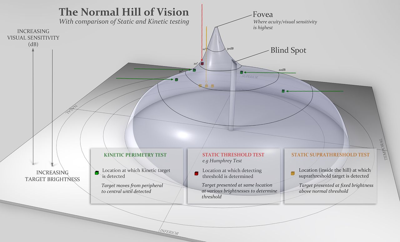
The fovea is the area of greatest visual sensitivity, where the cone photoreceptor density is at its highest. The visual sensitivity slopes off further from the fovea. This drop in sensitivity can be visualised as a hill, with the fovea is at the peak (figure 1). Conventional perimetry is carried out under photopic (well lit) conditions, and therefore, rod photoreceptors do not contribute to the findings.
The normal field of vision extends to approximately 60° nasally, 90° temporally, 60° superiorly and 70° inferiorly.
The blind spot indicates the location of the optic nerve head—an area with no photoreceptors—in the temporal part of the visual field.
Anything obstructing the travel of light towards the retina may affect the field tests, for example, lens opacity (cataract), ptosis (if not taped away from the pupil) or the rim of a correcting lens (test artefact)

Normal hill of vision.
Goldmann field test
During a Goldmann field test, the patient positions their eye opposite the centre of a white hemispherical bowl (figure 2). The patient fixates upon the central target 33 cm away, while the examiner sits opposite viewing through an eyepiece to ensure good fixation throughout the test. The examiner moves an illuminated white target from the periphery towards the centre, and the patient presses a buzzer to indicate when they first see the target. This is repeated from different directions—allowing the examiner to plot the patient's field of vision—using targets varying in size and brightness. The examiner plots the blind spot and the edges of scotomas in a similar way, with the patient pressing the buzzer to indicate when they first see the light target moving from a blind to a seeing area. The examiner also performs static testing—involving the brief appearance of the stationary light target—in the four quadrants within the central 20° or so, marking a tick on the chart when the patient sees the target and a cross if they do not.

Goldmann machine. The patient's eye is positioned at the centre of a white hemispheric bowl, with the examiner looking through an eyepiece to ensure good fixation. A white light (indicated by yellow arrow in (A) is brought in from the periphery into the patient's field of vision. The examiner does this by controlling connecting levers (indicated by orange arrows in A and B). The patient presses a buzzer when the light target is seen (blue arrow).
The target sizes are labelled with three alphanumeric digits, for example, ‘V4e’.
The first digit is a Roman numeral (I–V), indicating the size of the target, for example, V is equivalent to a target diameter of 9.03 mm. With every drop in number (eg, from V to IV) the diameter halves.
The second digit is an Arabic number (1–4), indicating the brightness of the stimulus: the larger the number the higher the luminance.
The third digit is a letter (a–e), indicating a finer calibration of luminance. ‘4e’ is equivalent to 10-decibel (dB) brightness; each consecutive drop in number represents a 5 dB change and each drop in letter represents a 1 dB change.
By convention, the examiner maps three isopters: lines of equal sensitivity to targets of a specified size and luminance. The first isopter, mapping the farthest peripheral vision, requires the largest and brightest target ‘V4e’. Another isopter is mapped in the central 30° of vision, and a third isopter is intermediate between these two. The isopter lines therefore show the margins of different visual sensitivity, analogous to the contour lines of a map marking different elevations. This allows us to visualise the hill of vision. The base of the hill represents the area at the periphery with least visual sensitivity, detecting only the largest and brightest target. As we move up towards the peak of the hill, the visual sensitivity increases and the patient sees smaller and dimmer targets.
Humphrey field test
The same principles apply to the Humphrey test as to the Goldmann test, but instead with static light stimulation. The machine can also be programmed to perform kinetic tests though we have no experience with this.
The illuminated targets appear for 200 ms at predetermined locations on a grid. Humphrey tests are widely used in glaucoma clinics, the most common set up being to test the central 24° (‘24-2’ setting). Some examiners test smaller or wider visual angles; however, the wider the visual angle tested, the more coarse the grid, and hence the greater the likelihood of missing small scotomas. The 24-2 assesses the central 24° with a 54-point grid; 10-2 assesses the central 10° with a 68-point grid; and 30-2 assesses the central 30° with a 76-point grid.
The examiner plots the hill of vision based upon the threshold for detecting different target luminance; as visual sensitivity improves towards the fovea, so the detection threshold for the target decreases. Unlike Goldmann, the target size stays the same during the test, with a default size equivalent to Goldmann size III targets. It is rare to need a different default size.
The Swedish interactive threshold algorithm (SITA) is the most commonly used test algorithm,3 designed to reduce the time to complete a test; a short test duration limits the likelihood of errors from patient fatigue. SITA starts by determining the visual stimulation thresholds at the four quadrants. If the patient sees the initial stimulus, the examiner reduces its brightness to the level where it is no longer seen. Conversely, if the patient does not see the stimulus, its brightness is increased to find this threshold. The examiner adjusts the initial brightness at adjacent points according to the threshold of its neighbouring point. During the test, the examiner retests some locations to determine reliability (see false-negative errors, below). At completion, the computer generates a statistical analysis, which is compared to an age-matched normal population.
Humphrey or Goldmann?
The choice may depend upon local availability. The Humphrey is slightly less operator-dependent than the Goldmann and has the advantage of numbers to indicate reliability of the test. The Goldmann tests peripheral fields better, may be more patient-friendly for those who are hesitant on the Humphrey, and is particularly useful for central scotoma, as it is easier to manage fixation losses. As a rule of thumb, when monitoring disease, it is sensible to use the same test as was used previously. Both tests can complement each other, confirming deficit patterns when in doubt.
Interpreting the Goldmann field test
The key to interpreting Goldmann visual fields is to keep in mind the normal hill of vision (figure 1) and how it compares with the patient's results. The skill is in identifying patterns and observing any change with repeated tests. This may require experience to be adept, though the following checklist may help (figure 3):
Patient name and date of test: a good habit always to check the test belongs to your patient!
What is the largest peripheral field (V4e)? This can vary according to age and test response. It normally extends to approximately 60° nasally, 90° temporally, 60° superiorly and 70° inferiorly. Thus, the superior aspect of the field is usually less sensitive than the inferior field, though ptosis could also artefactually reduce it.
Is there any distortion to the ‘contours’? (Contours are the smaller isopters corresponding to targets that are either smaller or dimmer or both).
Is the isopter smooth, as expected for a normal hill of vision?
Is there restriction? Examples would be a nasal step in papilloedema or an altitudinal defect in anterior ischaemic optic neuropathy.
Are the isopters spaced, as expected for the normal hill of vision? (1) A tiny central field with ‘stacked’ isopters—very close to one another as in a steep hill—usually denotes functional overlay (figure 7); however, patients with genuine retinal and striate cortex lesions may also have stacked isopters. (2) Isopter lines that cross always indicate unreliable test: isopters cannot cross since this would indicate two different sensitivities at one location. (3) Spiralling isopters suggest functional visual loss and indicate a steady decline in sensitivity during the test.
Are there scotomas? It is important to correlate this with the patient's symptoms and clinical (bedside) examination.
Is the blind spot size enlarged? This is particularly relevant in papilloedema (figure 5). The normal blind spot size is oval, roughly 10° in diameter, and located 10–20° temporally from the central fixation point.
Is the central field affected? Was static testing done (indicated with a tick when the patient saw the target)?
Is any defect monocular or binocular, when comparing the fields for each eye? If binocular, is the defect homonymous or heteronymous?
Any comments written about patient fixation or attention also help.
Small pupil size, ptosis and incorrect positioning of a correcting lens may affect the peripheral field.
Inadequate correction of refraction error for the viewing distance (33 cm) may affect the central field.

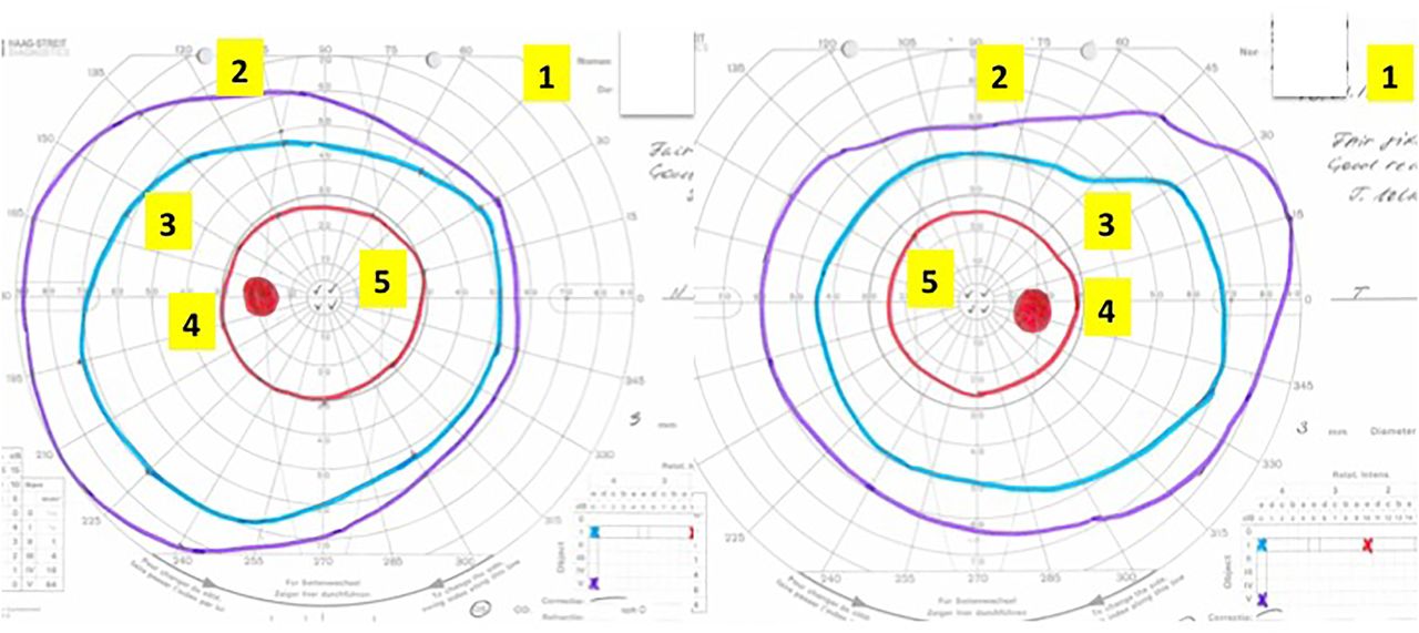
Interpreting the Goldmann visual field.
The chart is viewed from the perspective of the patient looking into the test bowl, as if patient is looking into the paper. Suggested checklist to review the Goldmann fields systematically (see text for details):
1. Patient name and identification number, date of test.
2. The largest isopter, that is, peripheral field.
3. The other isopters—any distortion to the ‘contours’ of the hill of vision? Any scotomas?
4. Blind spot.
5. Central vision.
6. If there is an abnormality, is it monocular or binocular? If binocular, is it homonymous or heteronymous?
7. Other, for example, comments about fixation or attention.
This is an example of normal Goldmann fields. In contrast, this patient did not perform well on the Humphrey visual fields, with poor reliability and cloverleaf pattern (figure 4).
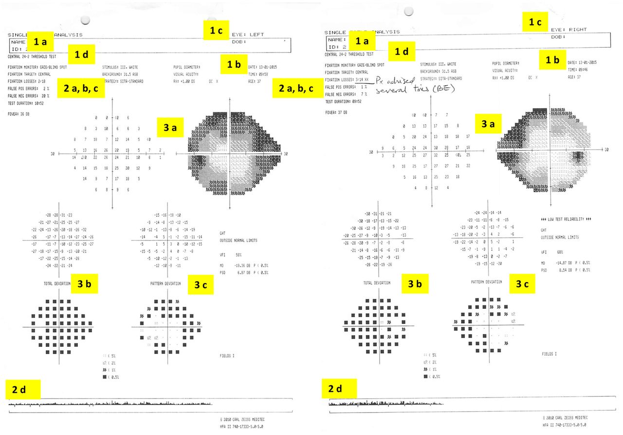
Interpreting the Humphrey visual field. The charts are viewed from the perspective of the patient looking into the test bowl, as if patient is looking into the paper. Suggested checklist to systematically review Humphrey visual fields (see text for details):
1. Is this the correct test?
A. Patient name and identification number
B. Date of test
C. Left or right eye?
D. Test performed
degree of visual angle tested
test protocol: threshold or screening
2. Can I rely on this test?
A. False-positive errors
B. False-negative errors
C. Fixation-loss index
D. Gaze-tracking graph
3. Is the test normal?
A. Visual sensitivity map
B. Total deviation map
C. Pattern deviation map
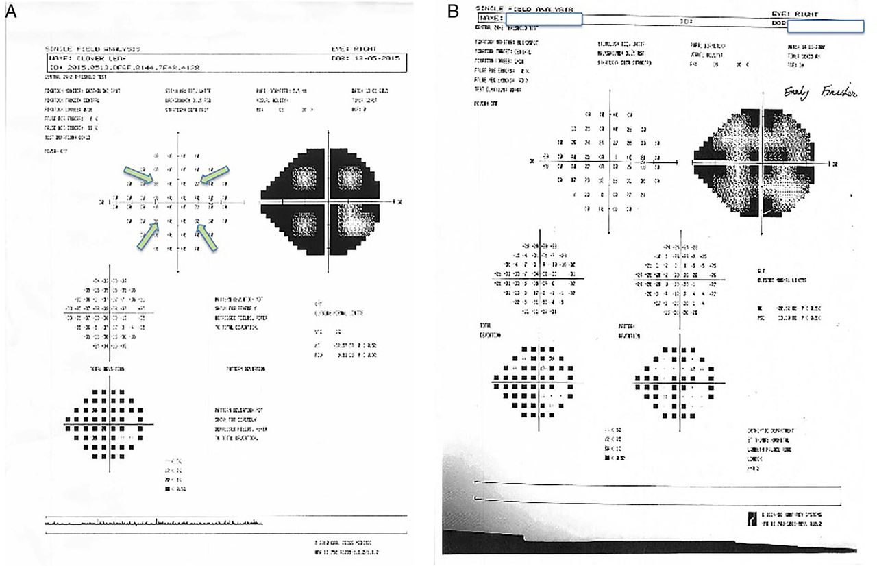
This patient's test was unreliable: high fixation loss index (and comment from technician, ‘patient advised several times for both eyes’ (suggesting poor compliance), gaze-tracking graph also showed eye movements (indicated by upward spike from baseline) and high false-negative errors, up to 20% in the left eye. The grey scale visual sensitivity map suggests a ‘clover leaf’ type pattern (figure 9). This provided the impression that the patient had difficulty with the Humphrey test itself. Clinical examination including visual acuity, colour vision, pupillary examination and visual field to confrontation to red pin was normal. The patient's Goldmann visual field test was normal (figure 3).

Goldmann visual field from papilloedema. This patient has papilloedema from idiopathic intracranial hypertension. Goldmann fields show (1) an enlarged blind spot and (2) inferonasal field restriction.

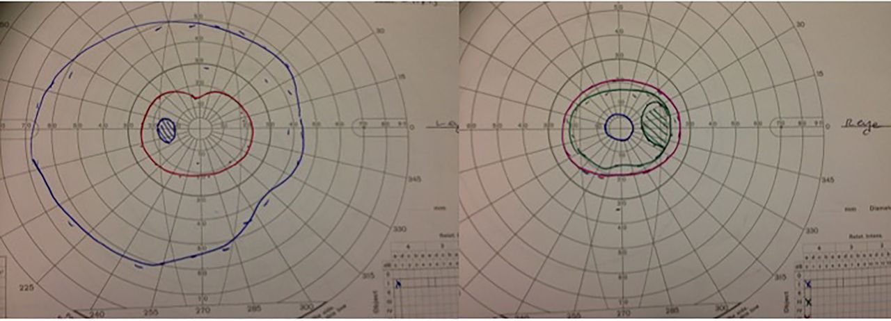
Goldmann visual fields of a patient with right optic neuropathy. All isopters are restricted but with preserved ‘contours’ of the hill of vision, giving the appearance of a ‘sunken hill’. Compare this with figure 7 showing stacked isopters in a patient with functional visual loss.

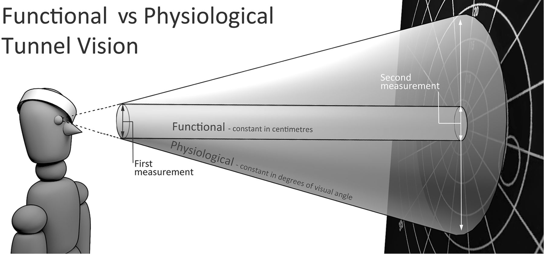
Goldmann visual fields of a patient with ‘stacked isopters’. This patient has functional overlay of a previous episode of mild optic neuritis affecting the right eye. Compare this with figure 6 of another patient with optic neuropathy. These ‘stacked isopters’ would represent a hill vision that is too steep to be physiological, that is, the close ‘contours’ here appear like a cliff drop. Clinical examination with a red target confirmed the presence of a tubular field (figure 8), with the size of visual field remaining unchanged when examined at 1 and 4 m. This is not keeping with the optics of light, whereby at a constant visual angle, the size of the field would appear larger the further away, that is, when examined at 4 m (with a proportionately larger target for acuity), the size of field to confrontation should be larger than on examination at 1 m.

Tunnel vision: functional (ie, tubular field) versus physiological. The optics of light is such that at a constant visual angle, the size of the field appears larger when further away. When examined at 4 m (with a proportionately larger target for acuity), the size of field to confrontation should be larger than on examination at 1 m. Thus, a ‘tubular’ field, where the size of field is unchanged, suggests functional overlay.

Cloverleaf pattern on Humphrey visual fields. This artefactual visual field defect results from a reduced response rate as the test progresses. The Swedish interactive threshold algorithm (SITA) threshold test starts by determining the initial brightness in the four quadrants using the four points indicated by the arrows. Therefore, if a patient's response deteriorates as the test progresses, for example, because of reduced concentration, the visual field shows a cloverleaf pattern, where the thresholds are low at the four points initially tested and higher for the surrounding points. This pattern commonly occurs in non-organic visual loss and is equivalent to ‘spiralling’ on the Goldmann. There will also be a high rate of negative errors. (A) Shows an example where the patient stops responding very early in the test, giving an extreme example of the cloverleaf pattern; (B) shows another example of cloverleaf pattern.
Interpreting the Humphrey field test
We suggest the following framework to interpret Humphrey test results (figure 4), structured to answer three questions:
1. Is this the correct test?
A. Name and patient number: confirm that the output belongs to your patient!
B. Date of test: is this the output of interest? that is, timing in relation to symptoms.
C. To which eye does this output correspond? Correlate the results with the history and clinical examination. Beware of fields that are mounted incorrectly: the conventional way of mounting is to place the left chart on the right and vice versa, ie, as if the patient is looking into the chart.
D. What test was performed? This is particularly important when comparing to any previous tests.
a. What degree of visual angle was tested?
Most commonly set to ‘24-2’ (central 24° tested with a 54-point grid). A smaller field with higher concentration of points gives further details of the foveal region. For example, ‘10-2’ assesses the central 10° with a 68-point grid. ‘30-2’ is similar to ‘24-2’ but with an additional 6° and with a corresponding increase in the points tested (76-point grid for 30°); thus, this is a longer test with the risk of more patient errors.
b. Was it a threshold or a screening test?
Screening tests use suprathreshold targets of single luminance and in the past were particularly useful because full threshold tests were time consuming. However, SITA threshold tests have superseded these, reducing test times (equivalent to the time taken for screening tests) without losing sensitivity.
2. Can I rely on this test?
A. False-positive errors
False-positive errors identify ‘trigger happy’ patients who respond in the absence of light stimulus. They are calibrated according to the patient's overall responses, therefore detecting when responses occur too soon after presenting a stimulus is. A false-positive rate of >15% compromises test results.4
B. False-negative errors
A false negative is the failure to respond to a relatively bright suprathreshold target in a region that previously responded to fainter stimuli. A high false-negative index may indicate hesitation or inattentiveness, though a true scotoma may also give false-negative results. However, in a true scotoma, the false-negative error rate is low for the contralateral (normal) eye.4 False-negative error may reduce with repeated testing as the patient gets used to the testing procedure.
C. Fixation-loss index
Fixation loss is tested by presenting a stimulus at the blind spot. If the patient sees this stimulus, it indicates loss of fixation. Values of >20% can compromise the test.4 However, this number could be artefactually elevated if the blind spot was inaccurately located, or in ‘trigger-happy’ patients. Tracking of the gaze (below) is better for assessing fixation loss.
D. Gaze-tracking graph
The eyes are tracked using video. The gaze tracking graph shows an upward spike when the eyes move and a downward spike when the eyes blink.
3. Is the test normal?
Three maps are generated with numbers and pictorial representations:
A. Visual sensitivity map
The numbers indicate the threshold of stimulus intensity detected in decibel (dB), with zero corresponding to the brightest intensity. Typical normal values centrally are around 30 dB. Values of 40 dB should not appear in standard test conditions but could occur in patients with high false-positive errors. The visual sensitivity may improve with repeat testing as patients become more familiar with it. The grey scale map is a visual representation of the numbers, with darker areas indicating poorer sensitivity to stimuli.
B. Total deviation map
This shows the deviations of the patient's visual sensitivity compared to an age-matched normal population. The numbers indicate the difference compared to the mean, that is, a negative value indicates less visual sensitivity compared to the mean population. The probability plot gives a visual representation of statistical analysis (t test) of this deviation from the mean; the larger departure from the mean, the darker the symbol.
C. Pattern deviation map
This shows the deviation of the pattern from a normal visual hill, where the peak is at the fovea. The numeric values show any departure from the mean of an age-matched population, and as above, the probability plot is a visual representation of statistical analysis indicating the extent of departure from mean. The pattern deviation adjusts for any shifts in overall sensitivity: for example, a patient with cataract might have a smaller or ‘sunken’ hill but with normal contour patterns.
By statistical chance, patients may have a few scattered dark symbols on the probability map, which may not be of concern. Instead, look for patterns, for example, whether these are around the blind spot, which might indicate a true enlargement. It is important to correlate the test results with the history and clinical examination.
The visual sensitivity, total deviation and pattern deviation maps should be viewed together for any discrepancies. It is worth noting the following scenarios:
Abnormal grey scale on stimulus intensity map but normal probability plots: lid partially obscuring the superior field.
Abnormal total deviation but normal pattern deviation: cataract, small pupils, incorrect correction for refractive error.
Abnormal pattern deviation but normal total deviation: a test with high false-positive (‘trigger happy’) patient.
Additional information that may help, especially when comparing with previous tests, include pupil diameter (is there a wide variation between tests?), lens modification (was the same correction used?), time taken to do the test (was this particularly long?). The global indices show the mean deviations, which can help to monitor progression, especially in glaucoma.
Three summary indices appear on the printout4:
The visual field index is a staging index designed to correspond to ganglion cell loss, that is, 100% represents normal fields and 0% represents blind fields.
The mean deviation represents the degree of departure of the whole field's average values, from age-adjusted normal values.
The pattern SD represents irregularities within the field, for example, of localised field defects. This can be small in completely normal patients or in those with complete blindness.
The visual field index and the mean deviation can help to identify progression; the visual field index may be less prone to artefacts from cataract. These values may help to monitor progression, but with caution, since artefacts and test reliability can affect them.
Conclusion
We present these simplified checklists to help neurologists to interpret Humphrey and Goldmann visual fields. We emphasise the importance of correlating these visual field outputs with careful patient history and clinical examination. Increased exposure to perimetry and its application in the clinical setting will help build up skills in its interpretation. For readers interested in deepening their understanding of fields and its nuances, we suggest further reading from the reference list.4–6
Key points
Perimetry results give a pictorial representation of the patient's ‘hill of vision’; keep the normal hill in mind when reviewing these tests.
Correlate perimetry results with the clinical history and examination (including examination to confrontation), as the tests often have artefacts.
Watch out for patient performance effect, for example, high false-positive or false-negative errors, cloverleaf pattern (static perimetry) or spiralling of fields (kinetic fields).
Perimetry results change if anything obstructs the travel of light towards the retina (eg cataract).
Static and kinetic perimetry complement one another; consider the other if the first is unexpectedly normal or abnormal.
Footnotes
Contributors SHW wrote the first draft of the manuscript; GTP reviewed and made revisions to the manuscript.
Competing interests None declared.
Provenance and peer review Commissioned; externally peer reviewed. This paper was reviewed by Mark Lawden, Leicester, UK.
Linked Articles
- Editors' commentary
- Miscellaneous
Other content recommended for you
- What do patients with glaucoma see: a novel iPad app to improve glaucoma patient awareness of visual field loss
- Agreement to detect glaucomatous visual field progression by using three different methods: a multicentre study
- Retinal nerve fibre layer assessment in myopic glaucomatous eyes: comparison of GDx variable corneal compensation with GDx enhanced corneal compensation
- Comparing the usefulness of a new algorithm to measure visual field using the variational Bayes linear regression in glaucoma patients, in comparison to the Swedish interactive thresholding algorithm
- Specificity of various cluster criteria used for the detection of glaucomatous visual field abnormalities
- Risk factors for microcystic macular oedema in glaucoma
- Ocular safety of sildenafil citrate when administered chronically for pulmonary arterial hypertension: results from phase III, randomised, double masked, placebo controlled trial and open label extension
- Pointwise linear regression analysis of serial Humphrey visual fields and a correlation with electroretinography in birdshot chorioretinopathy
- Bruch's membrane opening changes and lamina cribrosa displacement in non-arteritic anterior ischaemic optic neuropathy
- Comparing focal and global responses on multifocal electroretinogram with retinal nerve fibre layer thickness by spectral domain optical coherence tomography in glaucoma